The new FPS package
Latest update: March 2024
News
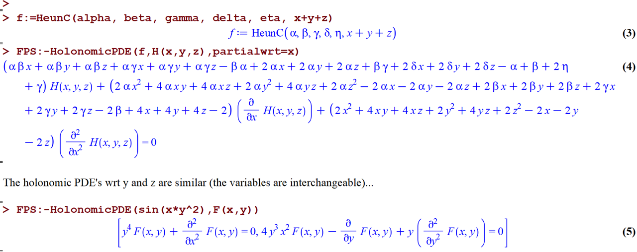
Multivariate D-finite functions: HolonomicPDE,(not to be confused with HolonomicDE, which we want to keep for the univariate case only) for computing holonomic partial differential equations from a given D-finite or holonomic expression. There are two main options:
partialwrt: called as FPS:-HolonomicPDE(f, F(x1,...xn), partialwrt=xk);
Computes a holonomic partial differential equation with respect to a variable xk for a given multivariate D-finite (holonomic in a sense) function f in x1, ..., xk, ..., xn. When no option is specified, the output is a list of n partial differential equations that can be used to write down a canonical representation of the input expression as a holonomic function.
elimvars: called as FPS:-HolonomicPDE(f, F(x1,...xn), elimvars=S);
Computes a holonomic partial differential equation with the variables in the set S, a subset of {x1,...,xn}, eliminated from the polynomial coefficients. An accompanying paper with the technique used behind is under preparation.
One can use FPS:-HolonomicPDE to compute specific annihilators and perform so-called telescoping in the differential case.
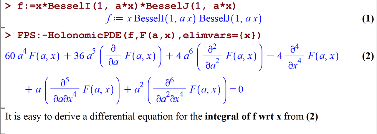
Eliminating x among the coefficients
D-finiteness
Introduction
FPS is a mathematical software for symbolic computations that provides tools for:
1- Computing homogeneous ordinary and partial differential equations for a large family of differentiable functions including meromorphic and special functions; henceforth deduce (in the ordinary case) recurrence equations for the series coefficients. The procedures are HolonomicDE, LinearDE, and QDE for differential equations; and FindRE, FindQRE, and sumhyperRE for recurrence equations. Finding the differential equation for the sums, products, and polynomial unary operations (like exponentiation and constant multiplication) of holonomic functions from differential equations that they satisfy: AddHolonomicDE, MulHolonomicDE, SelfOpHolonomicDE. For algebraic functions defined by polynomials, the procedure AlgtoHolonomicDE computes the least-order ODE.
2- Solving linear recurrence equations with polynomial coefficients by computing the basis of m-fold hypergeometric term solutions. The main procedure is mfoldHyper. There is also rectohyperterm which is a procedure for finding (1-fold) hypergeometric term solutions using a variant of Mark van Hoeij's algorithm.
3- Computing Formal Power Series, hence the name of the package. This is to find the power series representations of the so-called hypergeometric type functions (in closed form formulas) and non-holonomic functions by combining the procedures mentioned above. The resulting procedure is FPS which can be called without prefix.
4- And more: guessing (delta2guess), i.e, finding implicit or explicit representations of a sequence from finitely many of its terms. Note also the ongoing multivariate implementation of HolonomicDE.
As a byproduct, the package contains the procedure Taylor for computing series expansion for holonomic functions, and the procedure dispSet for computing the dispersion set of two given polynomials.
The acronym FPS was first used by Wolfram Koepf for his mathematical software which contains a variant of HolonomicDE, FindRE, and implementation for computing particular cases of hypergeometric type series. The software has been renewed by his former Ph.D. student Bertrand Teguia Tabuguia. Related articles are already published or under review.
FPS is implemented in the computer algebra systems Maple and Maxima.
Incorporation in Maple from the 2022 release:
FPS (the procedure) is convert/FormalPowerSeries
FPS:-mfoldHyper is LREtools:-mhypergeomsols
FPS:-HolonomicDE, FPS:-LinearDE, and FPS:-QDE constitute the core of DEtools:-FindODE
FPS:-dispSet is incorporated in LREtools:-dispersion
Download and use FPS
Click here to download FPS for Maple
The easiest way to use FPS in Maple is by putting the downloaded file, FPS.mla, in your working directory and include the lines
> restart;
> libname:=currentdir(), libname:
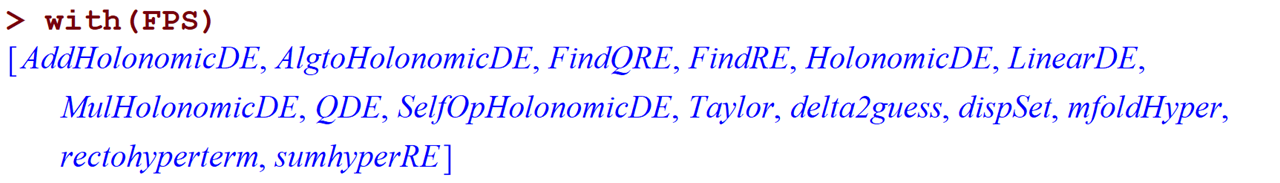
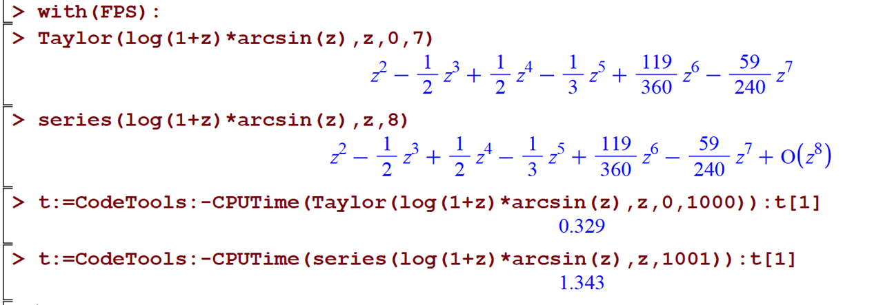
> with(FPS):
at the beginning of your worksheet.
However, to avoid carrying the file FPS.mla in all your working directories, you can just put it in a directory that you defined for libraries. For more details about this, please have a look at the Maple help page of libname.
Click here to download FPS for Maxima
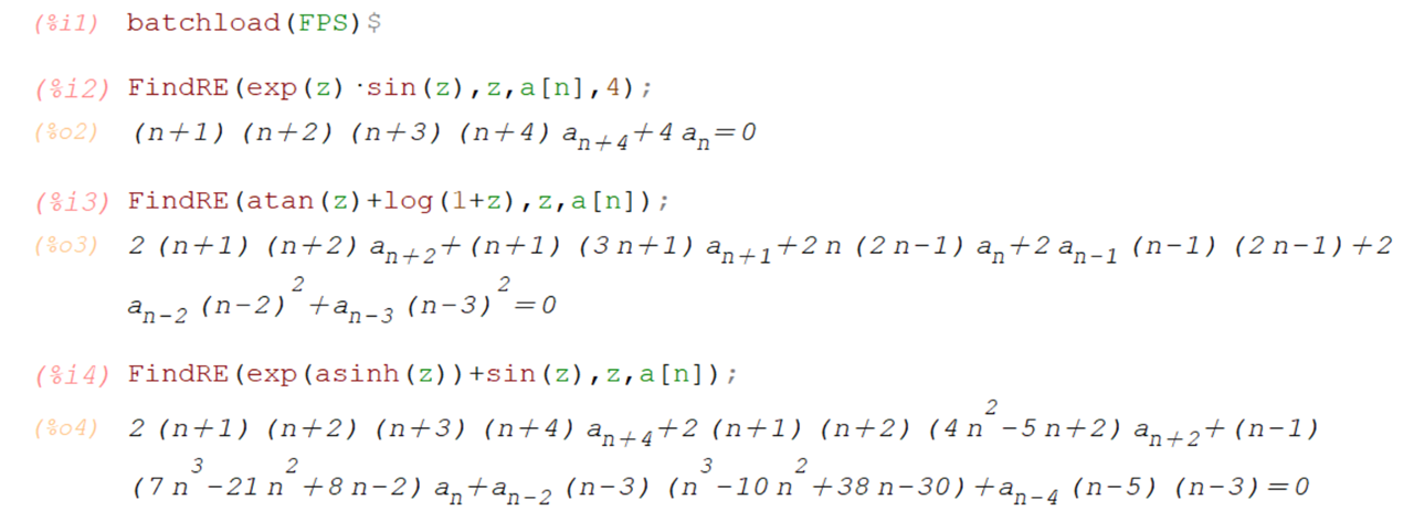
To use FPS in Maxima, you have to put the file FPS.mac in one of the directories listed by the Maxima global variable file_search_maxima, and load the package as follows
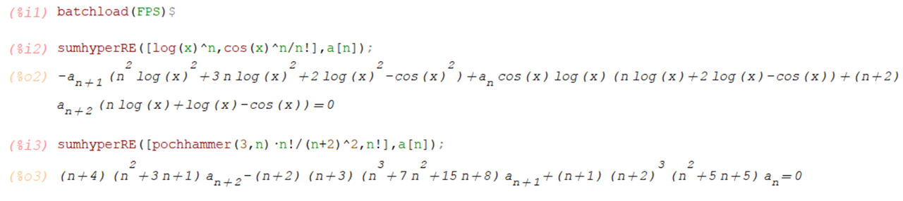
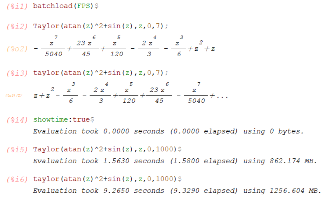
(%i1) batchload(FPS);
User guide of procedures
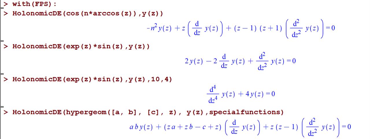
HolonomicDE(f,y(z))
Computes a holonomic differential equation satisfied by the function f in the dependent variable y(z) and the independent variable z.The default maximum order of the differential equation sought is 10.
In Maple:
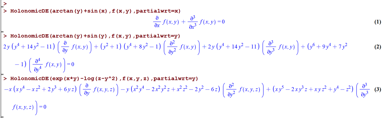
Recently added (September 2022): For computing a partial holonomic differential equation with respect to x_k for a given multivariate D-finite function f in x_1, ..., x_k, ..., x_n, one proceeds as follows:
HolonomicDE(f,y(x_1,...,x_n),partialwrt=x_k)
When the argument partialwrt is ommited, the output is a list of n holonomic partial differential equations that can be used to write down a canonical representation of the input expression as a holonomic function.
HolonomicDE(f,y(z),maxdeorder): maxdeorder most be a positive integer used to allow a larger value for the maximum order of the differential equation sought.
HolonomicDE(f,y(z),maxdeorder,destep): destep is a positive integer representing the minimum possible value of the difference between two derivative orders appearing in the computed differential equation. The default value is 1. The value of destep is only taken into account when maxdeorder is also specified. Common use: HolonomicDE(f,y(z),10,2), HolonomicDE(f,y(z),12,3), etc.
HolonomicDE(f,y(z),specialfunctions) or
HolonomicDE(f,y(z),maxdeorder,specialfunctions) or
HolonomicDE(f,y(z),maxdeorder,destep,specialfunctions):
(only for the Maple version) to be used when some special functions like hypergeom, Fibonacci, Bateman, JacobiP, etc. occur in f.
In Maxima:
The maximum order of the differential equation sought is controlled by the global variable Nmax whose default value is 10. The only optional argument is destep.
Partial holonomic DEs
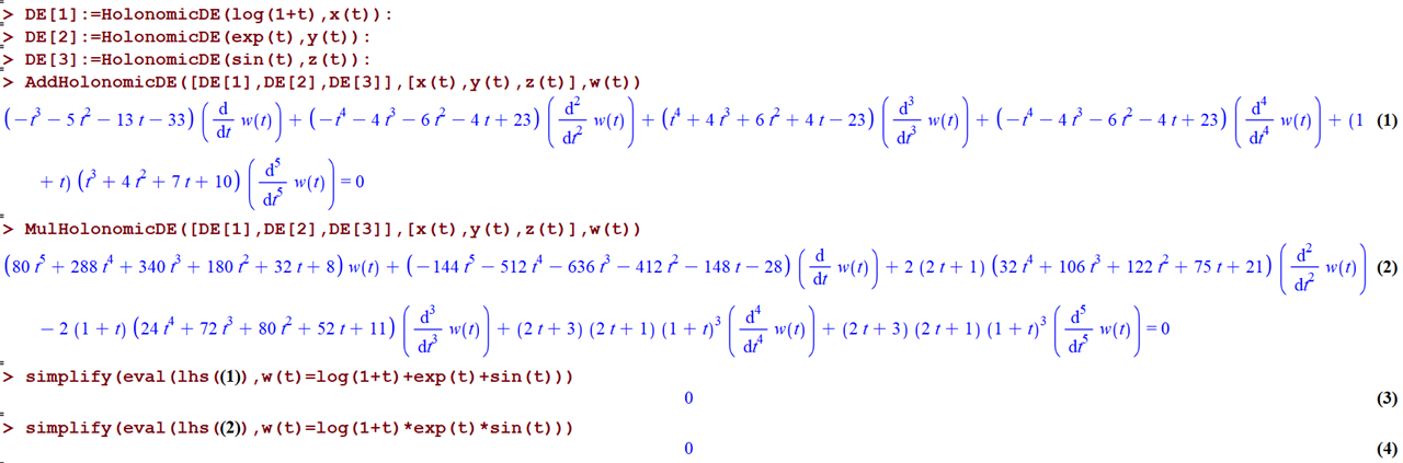
AddHolonomicDE(L,V,z(t)) and MulHolonomicDE(L,V,z(t))
Given a list of differential equations DE[i] in a list L, with dependent variables y[i](t) in the same order in a list V, the procedures AddHolonomicDE(L,V,z(t)), and MulHolonomicDE(L,V,z(t)) compute a differential equation for the sum of the y[i](t), and their product, respectively. The output is given using the dependent variable z(t). These procedures are currently only available in the Maple version.
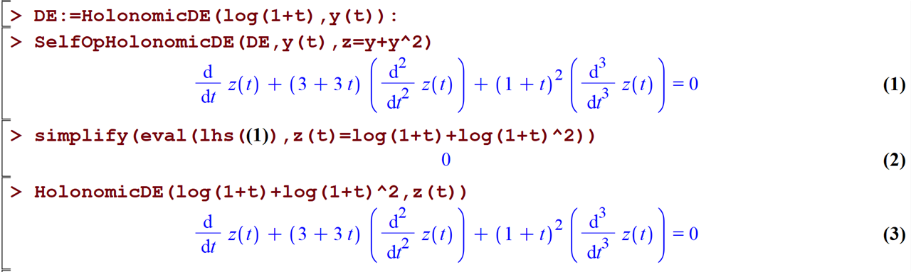
SelfOpHolonomicDE(DE,y(t),z=P(y)) (only in Maple)
Given a holonomic differential equation DE in y(t), computes a holonomic differential equation of a polynomial expression P(y) in y (y(t)).
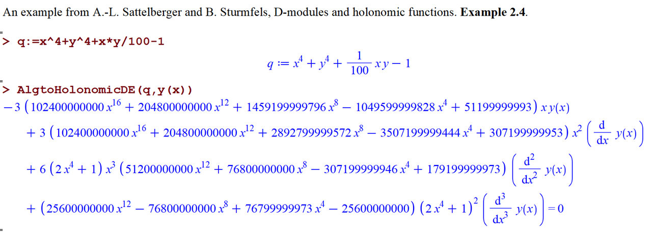
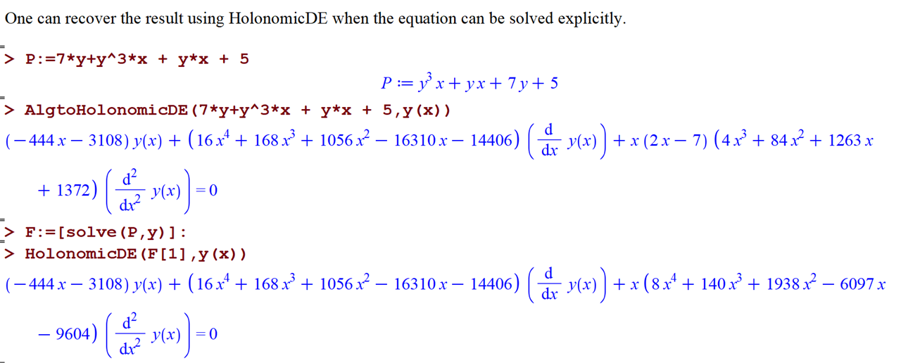
AlgtoHolonomicDE(P(x,y), y(x)) (only in Maple)
Computes the least-order (homogeneous) holonomic differential equation satisfied by y(x) from a polynomial relation P(x,y)=0 between y and x. The differential equation is valid for all non-constant solution y(x) of P(x,y)=0.
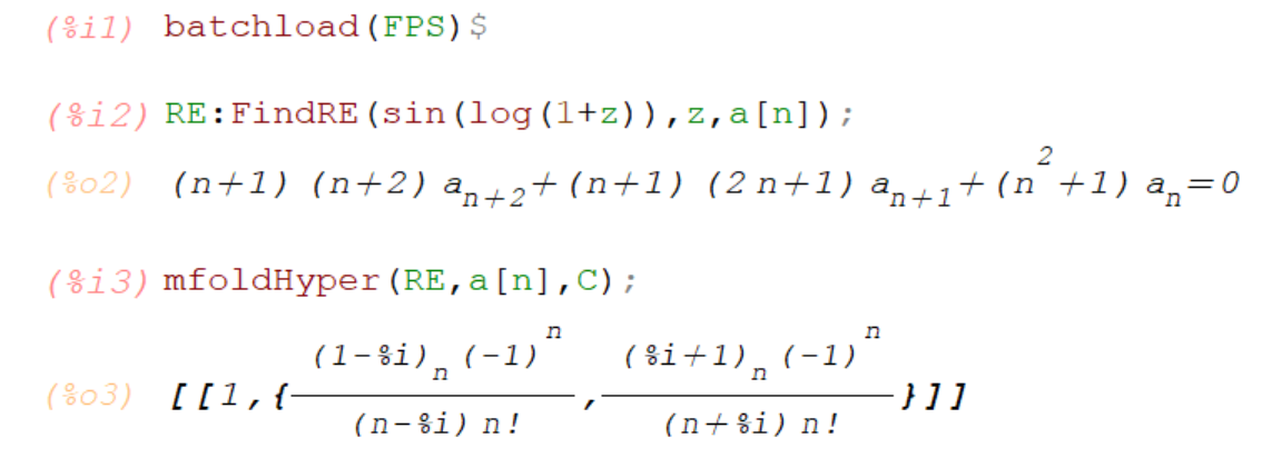
FindRE(f,z,a(n)) in Maple, FindRE(f,z,a[n]) in Maxima
Converts a holonomic differential equation computed by HolonomicDE into a recurrence relation. The optional arguments maxdeorder, destep, and specialfunctions are also valid for this procedure in Maple. In Maxima, only destep is considered.
The Maxima version provides the procedure DEtoRE(DE,F(z),a[n]) to convert any holonomic differential equation into a recurrence relation.
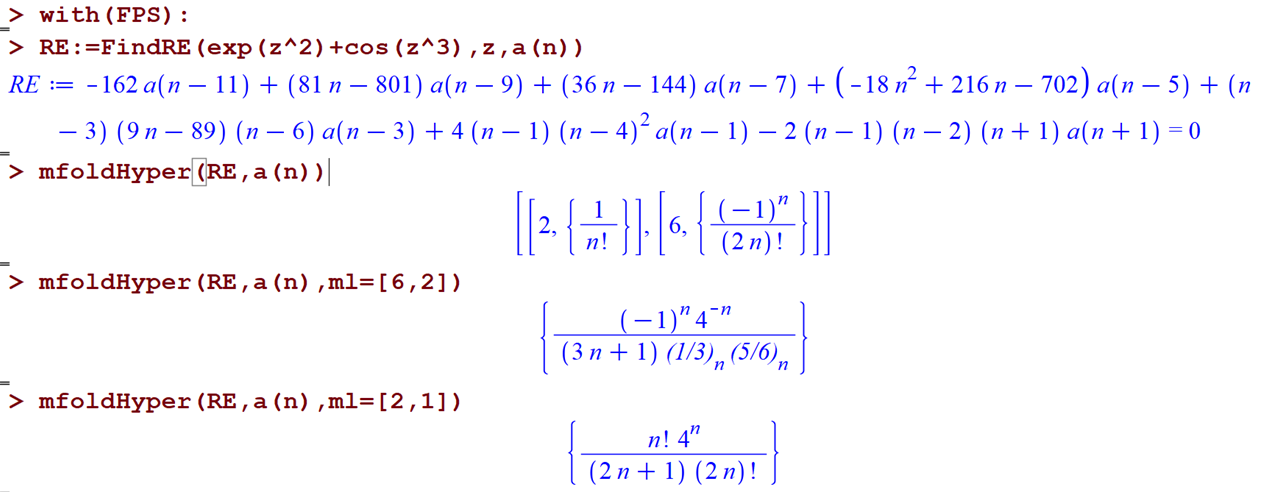
mfoldHyper(RE,a(n)) in Maple, mfoldHyper(RE,a[n]) in Maxima
Computes m-fold hypergeometric term solutions of holonomic recurrence equations. An m-fold hypergeometric term a(n) is such that a(n+m)/a(n) is rational over the considered field. The field of computation is controled by an optional argument. By default, the field of rationals (values and not symbols) is assumed. The output is a list of
[an integer m, set of m-fold hypergeometric terms].
mfoldHyper(RE,a(n),complex) in Maple
mfoldHyper(RE,a[n],C) in Maxima:
the computation considers algebraic extension fields, which includes solutions containing symbols.
mfoldHyper(RE,a(n),ml=[m,l]) or mfoldHyper(RE,a(n),ml=[m,l],complex) in Maple
mfoldHyper(RE,a[n],m,l) or mfoldHyper(RE,a(n),m,l,C) in Maxima:
to compute m-fold hypergeometric term solutions for a specific positive integer value of m and l, with m>l . The output is a set of m-fold hypergeometric terms.
rectohyperterm(RE,a(n)) in Maple, HypervanHoeij(RE,a[n]) in Maxima
works as mfoldHyper but only reduce to the case of (1-fold) hypergeometric terms.
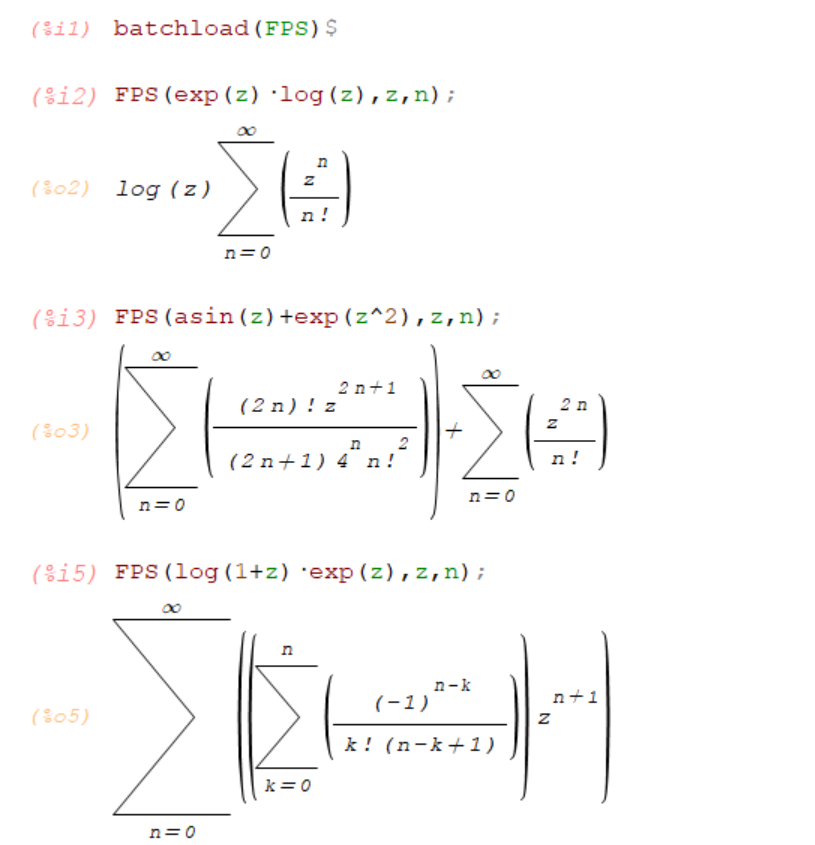
FPS(f,z,n)
Computes a closed-form formula for the power series representation of f in the variable z and the summation index n. The output is either a hypergeometric type series, or a recursive formula deduce from the recurrence equation satisfied by series coefficients.
Note that no prefix is needed for this procedure even when the package is not loaded (with(FPS)) in Maple.
FPS(f,z,n,z0): for expansion about z0.
By default, the procedure searches for a hypergeometric type series representation. If this is not found but a holonomic recurrence equation instead, then a recursive formula is given from that recurrence relation. Otherwise, a third approach base on computing quadratic differential equations is used.
In Maple:
FPS(f,z,n,onlyhyper=boolean): if boolean is true, then the computations stop once the search for a hypergeometric type power series is completed.
FPS(f,z,n,hypergeomcoeffs=true): to search for a hypergeometric type representation where every m-fold hypergeometric term solution of the underlying recurrence equation appears in a different summation.
FPS(f,z,n,fpstype=name): name can be 'holonomic', 'quadratic' or 'specialfunctions'.
holonomic: for deducing a recursive formula of the series from a holonomic recurrence equation. In Maxima, this is done using HoloRep(f,z,n).
quadratic: for deducing a recursive formula of the series from a quadratic recurrence equation. In Maxima, this is done by the QNF(f,z,n).
specialfunctions: to do the same computations when special functions appear in the input. This is not a proper optional method. The version incorporated in Maple does not need such a specification from the user since special functions can be detected by internal checking.
FPS(f,z,n,maxdeorder=M): To allow the search for a higher-order differential equation in order to have more chance in finding a representation of hypergeometric type or a holonomic recursive formula. This is done in Maxima by increasing the value of Nmax.
The Maxima package applied further techniques (Cauchy product, reciprocal of a series) to cover some other cases.

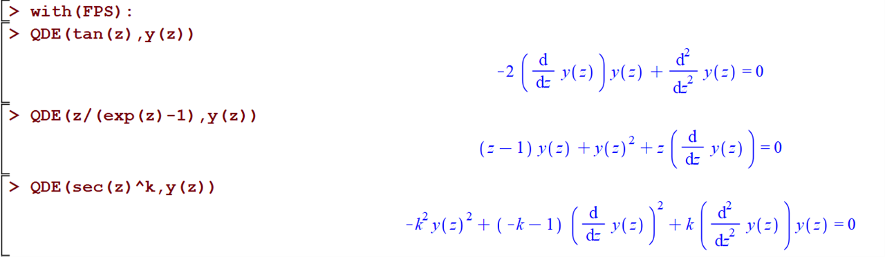
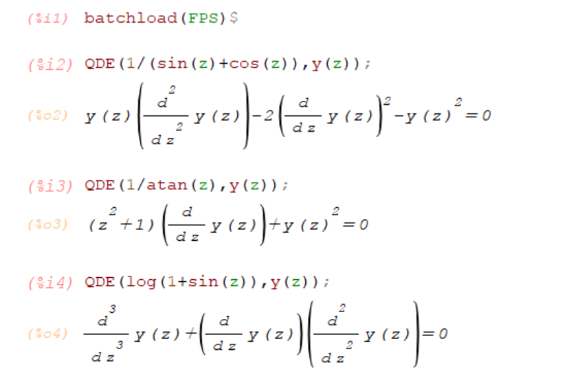
QDE(f,y(z))
Searches for a quadratic differential equation with polynomial coefficients, i.e. a differential equation which contains at most one product of derivatives (the square of a derivative is also included) in its summands.
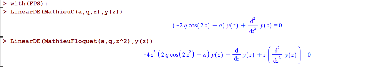
LinearDE(f,y(z)) (only in Maple)
A variant of HolonomicDE which allows some elementary functions as coefficients. This can be used to compute the differential equations for Mathieu functions for example.
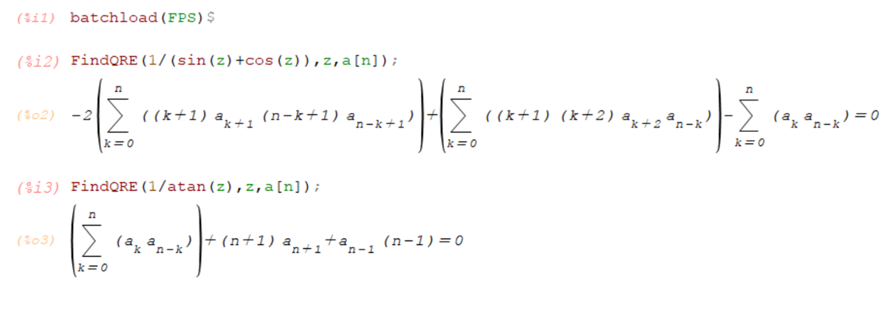
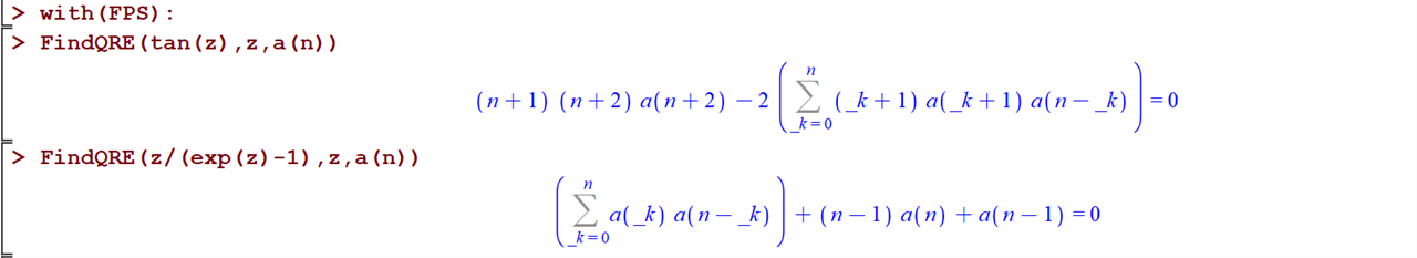
FindQRE(f,z,a(n)) in Maple, FindQRE(f,z,a[n]) in Maxima
Computes quadratic recurrence equations from quadratic differential equations computed by QDE.
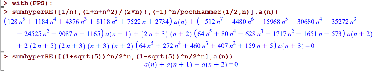
sumhyperRE(L,a(n)) in Maple, sumhyperRE(L,a[n]) in Maxima
Computes a holonomic recurrence equation satisfied by the sum of hypergeometric terms given the list L.
Taylor(f,z,z0,N)
Computes the Taylor polynomial of order N of the holonomic function f at the point of expansion z0. The used approach is based on holonomic recurrence equations and is more efficient for computing truncated Taylor series of larger-order.
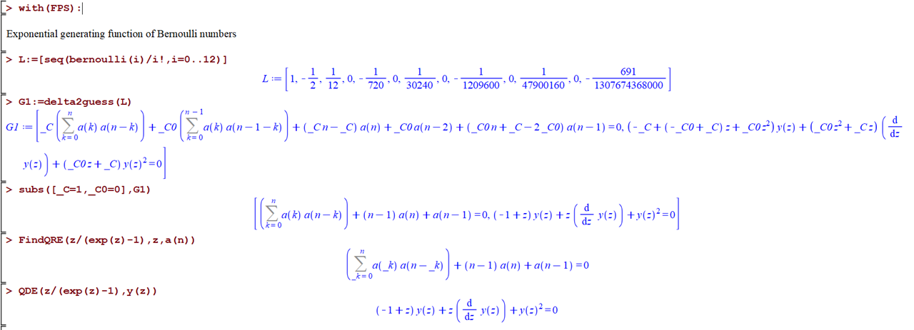
delta2guess(L,degpoly=d) (currently only in Maple)
Computes [RE, DE], where RE is a non-linear recurrence equation satisfied by the values in L, and DE is the corresponding differential equation that can be used to find the generating function of the values in L. The parameter degpoly (default value is 2) gives the degree bound of the polynomial coefficients.
This procedure mainly concerns sequences that cannot be defined by linear differential or recurrence equations like the Bernoulli numbers. The algorithm is quite fast since most differential equations in this category have polynomial coefficients with lower degrees.
For personal notation, one can use the optional parameters devars=[y,z] and revars=[a,n,k].